Author Archives: Manisha Sharma

This blog is the second post of a series of three blogs. In the  Previous Blog I had introduce the reader to the importance of forecasting “views” of an e-Commerce website. The process of forecasting can be implemented using the time-series approach and decomposing the “views” signal into four components namely seasonal, trend, cyclic and irregularity.

The decoupling can be achieved through exponential smoothing using the HoltWinters function of the forecast package of R.  After smoothing up the data the predict function can be fired to forecast the number of visits for the coming days. The output of the parameters (alpha, beta and gamma) will tell us the amount of weight that HoltWinters have put to recent and past data while minimizing the mean square error.

Implementing the time-series exponential smoothing in R:

I have used the HoltWinters (also a function in the forecasting package of R ) model to implement the exponential smoothing on the visitors data. You can get the resources for getting started with R here. This model will take care of the Seasonality, Trend, Cycling and Irregularity components of the time-series by adjusting the three smoothing parameters namely alpha, beta and gamma.

HoltWinters(x, alpha = NULL, beta = NULL, gamma = NULL)

Here, x is the time-series object which usually is a vector of the independent variable. (Number of visits for our example.)

Alpha is the smoothing parameter used for the estimation of the current underlying level. Value of alpha closer to 1 indicates that more weight is on the recent value of the independent variable and less on the previous data. And a value closer to zero is a forerunner that the model has put more weight on the past data for exponential smoothing.

Beta is for the estimate of the slope of the trend component at the current time point. This parameter of Holt-Winters filter specifies how to smooth the trend component. Like alpha it also runs from 0 to 1 where 0 means less weight on recent data and 1 means more weight is assigned to the new data.

The parameter gamma is used for the seasonality component which also runs from 0 to 1.

Setting the values of alpha= FALSE, beta=FALSE, gamma=FALSE will tell R that these components should be ignored while performing the smoothing. And setting them NULL will tell R to automatically select the appropriate values of these parameters by minimizing the mean square prediction error from one-stepped forecast.

Visits.csv is a Comma Separated Values file with the dimension “date” and the corresponding metric “#of visits” on that particular date. This csv file has been extracted from Google Analytics, through a package developed at Tatvic. You can download and get started with it here. The data is for two years, starting from Oct 2011 to Oct 2013. It has 731 data points, the following are the first four rows of the file “Visits.csv”.

library(forecast)
# It loads the forecasting package to R’s environment.
date_visits

Understanding the output:

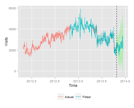
The above graph is the ggplot2 version of the plot function mentioned in the code described above.

The value of alpha (0.66) is relatively low, indicating that the estimate of the level at the current time point is based upon both recent observations and some observations in the more distant past. The value of beta is 0.00, indicating that the estimate of the slope b of the trend component is not updated over the time series, and instead is set equal to its initial value. In contrast, the value of gamma (0.81) is high, indicating that the estimate of the seasonal component t the current time point is just based upon very recent observations.

Let me recapitulate the gist of the post. I have used the HoltWinters function to implement the exponential smoothing for forecasting number of visits to a particular website. After smoothing up the data I have used the predict function to forecast the number of visits for the next 10 days. The output of the parameters (alpha, beta and gamma) will tell us the amount of weight that HoltWinters have put to recent and past data while minimizing the mean square error.

The next post in line is about detecting anomaly in the number of visits, using the concepts of upper and lower limit of the HoltWinters function, from the forecasting package of R.